
Edge vs. Fog vs. Cloud Processing: Latency Trade-off
Learn how latency deadlines, bandwidth, and compute limits determine where IoT functions should run: edge, fog, or cloud, with a worked example.
Contents & prerequisites
Every IoT system has to answer one architectural question before anything else: where does the data get processed? Push everything to the cloud and you get elastic compute and simple devices, but you pay in round-trip latency, bandwidth cost, and a single point of failure if connectivity drops. Push everything to the device and you get microsecond-to-millisecond response times, but you lose the aggregation, storage, and cross-site analytics that make IoT valuable. Edge, fog, and cloud processing are three points on that spectrum, and most industrial deployments split work across at least two of them, often all three. Getting the split wrong shows up directly as either unacceptable latency or unsustainable data and compute cost.
The Three Tiers Defined
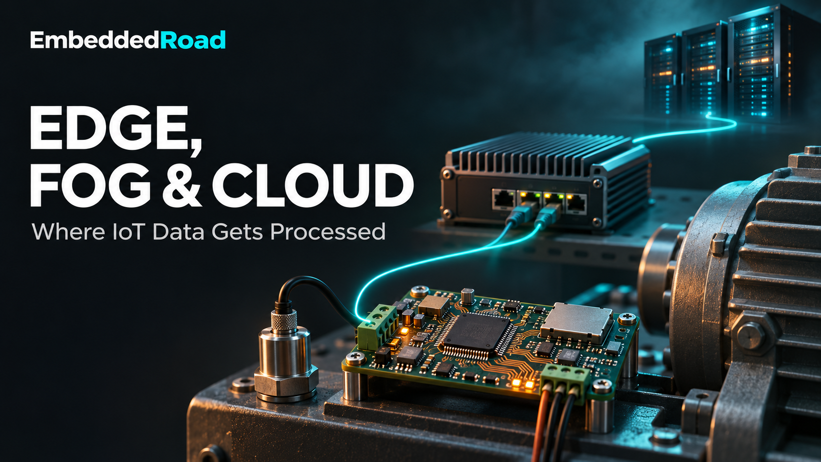
- Edge: processing on or immediately adjacent to the sensor or actuator — a microcontroller, a smart sensor with onboard DSP, or a single-board computer physically at the machine. Raw data stays local; only results, events, or summaries move up.
- Fog: processing on a local gateway, industrial PC, or on-premises server that aggregates multiple edge devices — typically within the same building, plant, or LAN. Fog sits between edge and cloud, doing filtering, local rules, and short-term storage before selectively forwarding to the cloud.
- Cloud: centralized compute in a data center, reachable over a WAN, offering elastic storage, heavy analytics (ML training, cross-site correlation), and long-term historical data.
The terms aren't always used with hard boundaries. "Edge computing" is sometimes used loosely to mean "not cloud," covering both edge and fog, and telecom operators use "edge" for multi-access edge computing (ETSI MEC) servers inside the mobile network, which sit between a plant's fog tier and a cloud region. The fog layer itself has a reference architecture, the OpenFog model adopted as IEEE 1934. For architecture decisions, the three-tier distinction is useful because each tier has a different latency budget, compute ceiling, and failure domain (see IoT device classification: constrained, gateway, cloud).
Latency Budget by Tier
| Tier | Typical response time | Compute available | Data volume seen |
|---|---|---|---|
| Edge (on-device) | ~1 µs – 10 ms, sensing to actuation | Limited (MCU/MPU class) | Raw, full-rate |
| Fog (local gateway/LAN) | ~1 – 50 ms, LAN round trip plus gateway processing | Moderate (gateway, industrial PC, or on-premises server) | Raw or pre-filtered streams from local devices, reduced before forwarding |
| Cloud (WAN) | ~10 – 100 ms over wired or LTE links to a nearby region; ~600 ms over GEO satellite; seconds over NB-IoT | Effectively unbounded, elastic | Aggregated, summarized |
These numbers assume edge latency is dominated by control-loop execution (interrupt to actuation); fog latency by local network hops — well under a millisecond on wired Ethernet, typically a few milliseconds on Wi-Fi with occasional spikes of tens of milliseconds — plus gateway processing; and cloud latency by WAN transit. LTE typically adds 30–70 ms of round-trip time before the internet hop (5G somewhat less), a geostationary satellite link about 600 ms, and LEO constellations tens of milliseconds.
Design against worst-case latency, not the typical figure. A cellular link that averages 40 ms can still stall for seconds during congestion, handover problems, or coverage gaps, and a deadline is only met if it's met at the 99.9th percentile and during outages.
Rule of thumb: a function whose deadline is shorter than the worst-case round trip to a tier, plus processing time there, cannot live in that tier. This is a hard constraint, not a preference — a motor over-current trip needing a 2 ms response cannot wait on a 100 ms cloud round trip no matter how much compute the cloud offers.
Worked Example: Motor Protection on a Factory Floor
A CNC spindle has three functions with very different time constants:
- Instantaneous over-current trip: must remove drive output within 2 ms of the current exceeding its trip level, to protect the drive's power stage and the motor. (A hard short circuit is handled faster still: the gate driver's desaturation detection turns the IGBTs off within microseconds. Thermal protection of the winding is a separate, much slower I²t function.)
- Vibration-based anomaly flag: should raise an alert within 1–2 seconds of an abnormal vibration signature appearing — chatter, imbalance, or a jump in bearing-defect frequencies.
- Fleet-wide predictive maintenance model: retrains weekly across 200 machines using months of vibration and temperature history.
Mapping each to a tier:
- Function 1 → Edge. A local ADC plus comparator/MCU loop sampling at, say, 10 kHz has a 100 µs sample period, so detection and shutdown within 2 ms are achievable entirely on-device; in practice a hardware comparator in the drive does it in microseconds (see gate drive: bootstrap, optocoupler, isolated ICs). Sending this over any network — even a 1 ms LAN hop — adds risk with zero benefit, since the actuation must happen locally regardless. Where the trip is part of a safety function, it belongs in the drive's certified safety logic (for example, Safe Torque Off per IEC 61800-5-2), not in an IT tier.
- Function 2 → Fog. The shop-floor gateway receives the raw vibration streams from 20 spindles over the plant LAN — 5 kHz × 3 axes × 16 bits = 240 kbit/s = 30 kB/s per machine, about 4.8 Mb/s for all 20, trivial for Ethernet — computes FFT features, and runs a lightweight anomaly classifier. Most of the 1–2 s budget goes to the analysis window, not the network: a 4,096-point FFT at 5 kHz spans about 0.8 s of data (≈1.2 Hz resolution), while the LAN adds milliseconds and the classifier about 100 ms. Keeping this in the fog also keeps the raw stream off the WAN. For high-speed spindles, bearing-defect analysis with envelope demodulation often needs sampling at 20 kHz or more, which makes the raw stream several times larger and the case for local feature extraction stronger.
- Function 3 → Cloud. Weekly retraining needs months of history from all 200 machines and GPU-class compute, which the cloud provides elastically (an on-premises GPU server is the alternative where data must stay on site), and a 500 ms round trip is irrelevant at a weekly cadence. The fog tier forwards only extracted features — about 1 kB/s per machine instead of 30 kB/s — and the retrained model is pushed back down to the gateways, which run the inference (see CI/CD pipeline for edge AI model deployment).
Check: raw data per spindle is 30 kB/s ≈ 2.6 GB/day. Across 200 machines that's about 520 GB/day if sent raw to the cloud — roughly 48 Mb/s sustained around the clock, half of a 100 Mb/s plant uplink, and about 15.6 TB a month to store. Fog-side feature extraction cutting this to 1 kB/s per machine drops the WAN load to about 17 GB/day fleet-wide, a 30× reduction, while the 2 ms trip function never touches the network at all. The split is what makes the numbers work; no single tier could satisfy all three constraints alone.
Why Not Just Use the Cloud for Everything
- Physical response time: control loops with millisecond deadlines cannot tolerate WAN jitter, which is often larger than the deadline itself.
- Bandwidth cost: raw sensor streams (audio, vibration, video) are orders of magnitude larger than the events derived from them; in deployments with high-rate sensors, moving and storing raw data (cellular data, cloud ingestion, storage) is often the largest recurring cost.
- Availability: a WAN or cloud outage must not stop a safety-critical local function. Edge and fog tiers must be able to operate autonomously (degraded mode) when the uplink is down, and safety functions shouldn't depend on the fog tier either.
- Privacy/regulatory: some data (e.g., health data, video with faces) may be required to stay on-premises or be anonymized before leaving the site.
Why Not Just Use the Edge for Everything
- Compute ceiling: MCUs and even edge MPUs can run compact, quantized models, but not large models, and they can't train them. A gateway-class device can store months of its own data, but not the fleet's.
- Fleet-wide visibility: a single machine's edge controller has no way to see patterns across 200 machines — that requires aggregation, which is the fog or cloud's job.
- Update/maintenance cost: pushing analytics logic to thousands of distributed edge devices is harder to version and debug than centralizing it, and every change becomes a fleet update (see IoT device management: registration, monitoring, OTA).
Design Implications
- Classify each function by its worst-case deadline first, then place it in the most centralized tier that still meets that deadline, and move it down only when bandwidth, availability, or privacy require it — not to whichever tier is most convenient to develop on. Pushing a function down a tier (edge instead of fog) tends to reduce latency and network dependency but increases per-device cost and update complexity; pushing it up a tier does the opposite.
- Fog shapes what reaches the cloud. Besides local decisions like function 2, its biggest architectural job is usually data reduction — filtering, downsampling, feature extraction, and buffering during WAN outages — so the cloud only sees what it actually needs.
- Design for graceful degradation. Edge and fog tiers need a defined offline behavior (e.g., last-known-good setpoint, local alarm buffering) for when the cloud is unreachable, rather than assuming connectivity. Buffered data should keep its original timestamps and be forwarded when the link returns.
- Re-evaluate the split as models and hardware evolve. Increasingly capable edge and fog hardware (NPUs on gateways, quantized ML on MCUs) keeps pulling functions that used to require the cloud, such as simple anomaly detection, down to the fog or edge (see edge AI vs cloud inference). The boundary is not fixed; it shifts with silicon capability.
Key Takeaways
- Edge, fog, and cloud trade latency against compute and storage capacity: edge is fastest but weakest, cloud is slowest but most powerful, and fog sits in between, typically doing local decisions and data reduction.
- Latency deadlines are a hard constraint: a function must live in a tier whose worst-case round trip, plus processing, is shorter than its required response, regardless of available compute elsewhere.
- Place each function in the most centralized tier that meets its deadline, then move it down only for bandwidth, availability, or privacy reasons.
- Bandwidth and cost, not just latency, drive the edge/fog split: raw high-rate sensor data is usually reduced to features or events before it reaches the WAN.
- Most industrial systems split functions across several tiers at once, based on each function's own deadline, rather than adopting one tier exclusively.
- The boundary moves over time as edge and fog hardware grows more capable, so architecture reviews should periodically re-check which tier each function actually needs.
Learning
Sign in to track your progress.
Evidence
Public projects engineers linked to Edge vs. Fog vs. Cloud Processing: Latency Trade-off.
No engineer has linked a project to this topic yet. Built something that proves it? Add the project and tag it with iot-connectivity-edge-vs-fog-vs-cloud-processing-latency-trade-off — it then shows here and on your public profile.